Towards making Maths Understandable.

Towards making Maths Understandable.

Mathematicians as researchers need to better attend to communicating not just their definitions, theorems, and proofs, but also their ways of thinking:

“Mathematicians who don’t spell out the details of their work are like climbers who reach the top of a mountain without leaving hooks along the way. Someone with less training will have no way of following it without having to find the route for themselves,” Katrin Wehrheim

This need for more clarity should be reflected in both their teaching of mathematics and in the communication of their research. Is it possible to reconcile into one mode of expression of understanding  both the teaching method and the practice of doing Mathematics?

We need to appreciate the value of different ways of thinking about the same mathematical structure. We need to focus far more energy on understanding and explaining the basic mental infrastructure of mathematics, with consequently less energy on the most recent results. This entails developing mathematical language that is effective for the radical purpose of conveying ideas to people who don’t already know them. (On proof and progress in mathematics, William P. Thurston)

Consider in turn, issues related to teaching and then the expression of doing mathematics given that its apprehension is recognised as following one of two modes of understanding,(David Wees):

Relational mathematics (‘knowing both what to do and why’) consists of building up a conceptual structure (schema) from which the student can produce an unlimited number of plans for getting from any starting point within that schema to any finishing point.

“You can’t plough a field by turning it over in your mind.” ― Gordon B. Hinckley

In contrast, instrumental mathematics (‘rules without reasons’) consists of the learning of an increasing number of fixed plans, by which the thinker can find their way from particular starting points to required finishing points deigned the answer to the questions. The plan is algorithmic enunciating what to do at any stage of the process.

Therefore teaching delivery may elicit two kinds of teacher-student mismatches, (Richard Skemp) :

1. A learner satsified to understand instrumentally, guided by a teacher (and book) who wants them to understand relationally.
2. A meta-cognitive learner whose goal is to understand relationally, guided by a teacher who provides instrumental instruction.

The first of these will cause fewer problems short-term to the student, but it will be frustrating to the teacher. The latter is more damaging to the student especially when it is effected from a written text.

A cautionary note from Cognitive Load theory

Cognitive Load Theory, CLT tells us, why-students-make-silly-mistakes-in-class-and-what-can-be-done. Unlike “learning styles” theory, there seems to be a lot of research backing problems in overloading pupil’s RAM! CLT suggests that the bottom-up incremental, instrumental approach is the best way to develop a pupil’s appreciation of the methods of mathematics. At least to build up their confidence to motivate more self-driven enquiry. CLT suggest that any Big picture, relational teaching is perhaps an indulgence of the teacher; yes they can connect a few dots and create some narratives to motivate example but for the most part this top-down view comes from within the learner over time.

Herein lies the conflict. Thurston’s quote suggests that it is the relational way of understanding that mirrors the mathematical research method we as teachers should employ rather than the instrumental mode.

We look next at how either of the modes sit with the public perception of what actually is this business of doing mathematics.

What is the Study of Maths?

There are two conceptions of mathematics, the currency of mathematics is:

•  ideas
• proofs

The latter mindset says that the study of mathematics involves an abstract deductive system consisting of:
1. A set of primitive undefined terms;
2. Definitions evolved from the undefined terms;
3. Axioms or postulates;
4. Theorems and their proofs.

A public understanding caricature of mathematics is the Definition-Theorem-Proof (DTP) model which reads as follows:
Define.  mathematicians start from a few basic mathematical structures and a collection of axioms “given” about these structures,
Theorise.   there are various important questions to be answered about these structures that can be stated as formal mathematical propositions,
Prove.   the task of the mathematician is to seek a deductive pathway from the axioms to the propositions or to their denials.

The instrumental teaching mode involves the modelling of the solving of a problem and then the rolling out of problems with variations of minimal differences for the students to apply themselves and plays to this algorithmic theme.

A clear difficulty with the DTP model though is that it fails to beg the student to be curious of the source for the questions. A complete description of what mathematics is at the practitioners level must include such Speculation: the making of conjectures, the raising of questions, intelligent guesses and heuristic arguments about what is most likely to be proven to be true.

“Someone’s sitting in the shade today because someone planted a tree a long time ago.” ― Warren Buffett

A measure of increased success in the understanding of the field could thus be expressed by the extent to which successive researchers and interlopers apprehend and understand mathematics in its fully relational form.

Mathematical Objects by Association

While students may approach a piece of mathematics from one tentative viewpoint, practising mathematicians will understand the concept in multiple ways.

People have amazing facilities for sensing something without knowing where it comes from (intuition); for sensing that some phenomenon or situation or object is like something else (association); and for building and testing connections and comparisons, holding two things in mind at the same time (metaphor). These facilities are quite important for mathematics. ( William P. Thurston)

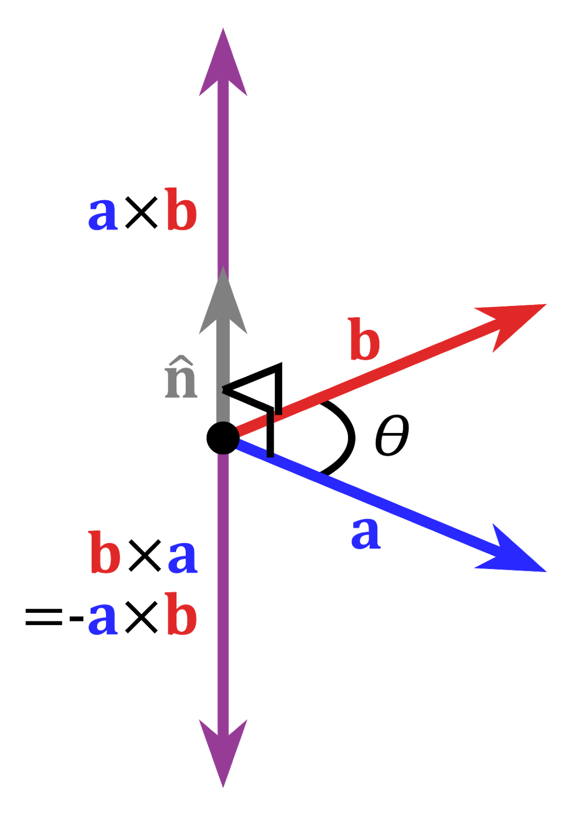
Consider the notion of a vector. To communicate the idea to students you might consider giving examples of vectors in the abstract and then instances of how they are realised kinematically in nature. A vector is then:

1. a directed line element/segment – usually represented by an arrow whose head type indicates its kinematical form in the field of mechanics,
2. has as archetype the position vector – an orientated directed distance from the origin of some arbitrary co-ordinate axis that enables the location of the head of the arrow to be determined by the tuple (x,y) in which the base of the arrow is at (0,0)
3. a displacement vector of relative positions
4. the (absolute/relative), (instantaneous/average) velocity vector, being the rate of change of those various types of displacement.
5. the absolute acceleration vector as the rate of change of velocity or indeed the snap of the relative acceleration.

That these are vectors objects and not scalar ones can be made clear by saying that non-examples of vectors are:

1. distance, speed
2. Temperature, Pressure as Real number Field values

And then you might want to consider why there is no scalar equivalent of acceleration. Such mapping of physical quantities to their algebraic symbols then helps uncover common student errors such as setting vectors equal to scalars, or comparing finite quantities with infinitesimals. Interpreting Derivatives, Dray et al. Of the latter consider then the notion of a derivative:

1.  Physicists: A ratio of (very)  small changes in quantities?
2. Mathematicians would consider the slope of the tangent line that is the limit of the slopes of secant lines?The average rate of change, no matter how small the domain, is different from an instantaneous rate of change.

The physicist would ask: How does one take the limit of discrete, numerical data, such as that measured during an experiment and Calculus then becomes less about the formal limits of “analysis”, rather more the art of infinitesimal reasoning: quantities that are “small enough” for the purpose at hand.

Students do not distinguish between the graph of the function and the graph of the function’s rate of change which might be attributable to students not conceiving of rate of change as a quotient of two quantities, discussing the rate of change as a slope but not speaking of slope as a quotient (the change in a function’s value being so many times as large as the corresponding change in its argument). Instead, they talk about slope as the function’s steepness. As another example, students often use a tangent line and rely on visual judgments to sketch the derivative function. Interpreting Derivatives, Dray et al

In increasingly more developed mathematical language the derivative can be thought of as ( William P. Thurston):

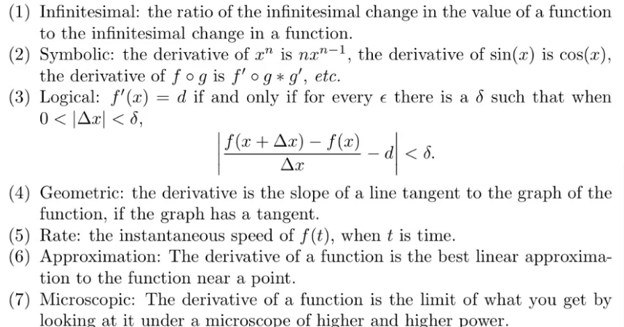
This is not just a list of different logical definitions but rather a list of different ways of thinking about the derivative. Only by embracing the Relational mathematics viewpoint, making contact to tangible instantiations of otherwise increasingly more abstract conceptions will the student be able to apprehend higher order abstractions by building on longer term retained and bedded down comprehensions.

Relationism is the Categorising of Equivalences

As you learn more and more math, your brain will run out of room if you don’t use category theory to organize your knowledge. And once they get deep enough into category theory, most mathematicians realize it’s a lot of fun. It’s very clean, very conceptual, and impossible to forget once you understand it. John Baez

At a higher level, an appreciation of the interplay between the objects of mathematics and their physical realisations as a route to understanding may be gained by considering the primary differential geometric object of Einstein’s General Relativity (GR). Within the freely falling (elevator) framework of GR we have,

Physical coordinates in different reference frames are related by Lorentz transformations (as in special relativity) even though those frames are accelerating or exist in strong gravitational fields. (Physical time and physical space in general relativity, Richard J. Cook)

The defining object of Einstein’s GR, then is an observational platform consisting of a network of laser-based stopwatches and rulers measuring Einstein’s falling elevator in an ambient gravitational field. Specifically the frame field is defined as a collection of observers distributed over space and moving in some prescribed manner. Each observer, (” local witness”), O is assigned space coordinates  that do not change. The Os are ‘‘at rest’’ ( ) in these coordinates. Each O carries a standard measuring rod and a standard clock that measure proper length and proper time at his/her location. The basic data of GR are the results of local measurements made by the Os.

This object can be traced alternatively from Gauge theories in which an equivalence class of bosons fields gives rise to a uniquely realised (vector) gauge boson excitation through the Gauge Principle. The underlying Gauge Equivalence maps to Einsteins’ Equivalence Principle. This later developed Gauge Principle itself applied by Yang-Mills rather pertained to the three non-gravitational forces effectively realises a soldering form object that knits together the local flat Lorentzian space of Special Relativity with the global co-ordinate diffeomorphism invariance principle of GR.

Relationism is everything in mathematics, category theory is telling us here that the soldering form is a functor mapping the locally equivalent gravitational and inertial viewpoints as espoused by the Equivalence principle. By employing this “gauge” object rather than the “metric” object of Einstein, Mathematicians can then see further equivalence between gravitational and non-gravitational interactions that would otherwise appear distinct in their nature.

What is the Plan Stan?

From those that appear to know, on the virtues of planning your means of communicating:

“Plans are of little importance, but planning is essential.” ― Winston Churchill

“Give me six hours to chop down a tree and I will spend the first four sharpening the axe.” ― Abraham Lincoln. ‪

Both recognise that drawing together relationships rather than collating a bunch of mere blunt instruments is more fruitful in the long run. I have not achieved this here by any stretch, but the template from How to give a great research talk seems like a reasonable structure to follow:

1. Abstract (4 sentences)
2. Introduction (1 page)
3. The problem (1 page)
4. My idea (2 pages)
5. The details (5 pages)
6. Related work (1-2 pages)
7. Conclusions and further work (0.5 pages)

Note here that related work comes as number 6 not number 3 in the list, a feature of some many educational articles that in trying too hard to justify the earnest of their efforts, lose the reader in a myriad of cross-referential tag teaming.

Above all endeavour to plan to make your mathematical expositions relational in content no matter how intrinsically abstract or abstruse that may be.

What is Equilibrium?

I always had a problem understanding coarse-graining: Macroscopic state variables such as Temperature represent, say aggregate molecule speeds within cells that are homogenous enough in character at a certain coarseness of scale.

These cells are localised islands of tranquility and we stitch them together. But that very choice of scale implies no equilibrium exists between neighbouring islands; if not why not make the view coarser and broaden the cell?

The cells otherwise are transitioning according to the zeroth law, being in mutual contact as they are at different aggregate temperatures.

So is not one observers coarse-grained view of a system of localised states in static equilibrium another ones view of states still in flux? Equilibrium is scale-dependent?

Handedness in Physical theories

Linear Operators and Oriented Parallelepiped

In Middle school we are asked to solve a pair of simultaneous equations perhaps with the motivation that those linear equations represent some crossing of trajectories in space and that in solving the set we are determining where an intersection takes place.

Such a set of equations: 5x- 2y= jx and -2x+2y=ky can be represented as a matrix equation. With two free parameters, j and k for two equations we have a suite of possible solutions for the different lambda. Recast in this matrix form our system of simultaneous linear equations is an eigenvalue problem with  eigenvalues 1 and 6. The solution to a pair of simultaneous equations thus describes a parametrised suite of straight lines.

The set describes straight lines with a variable gradient, m=(5-j)/2 or 2/(2-k). The simultaneous equation is configured as a matrix, A operating on a column vector, x. The eigenvalue problem asks for a pair of straight lines (from the infinite set of possible two straight lines intersecting at the origin), which are orthogonal to each other. That they are perpendicular means that the eigenvector solutions describing the lines are at right angles, thus linear independent forming a vectors basis.

Operationally, to find this linear independent set of eigenvectors that span the space of solutions we
take the determinant of the matrix A (denoted by |... |). As a set of solutions, all other possible solutions are mere combinations of these bases vectors. In our example the eigenvalues are 6 an 1 which tells us that the eigenvectors are (-1,-2) and (-2,1) or (4,-2) and (-2,-4). We can roughly think of matrices as operators (in a particular basis) that act on vectors, quite generally  rotating, stretching, compressing or displacing them in space. Eigen-vectors are special column vectors that when acted upon by such matrices merely react by stretching or compressing (mathinsight.org)  in length.

In Quantum (Linear) Mechanics these Linear operators give rise to the observables (vector) states that we see as the s and p shell eigenvalues of an atom. Linear Operators mark out the energies of the atom's states.

Geometrically what we are doing in looking for Eigenvectors, is to find the set of vectors that span our solution space - that is from which we can, for example, form a mutually orthogonal bases set of which all other solutions are a mere combination of such base factors.

We could envisage any number of such equations to solve and quite generally we could have a set of n simultaneous equations, with n unknowns.  We have abstracted our familiar world of the space of two-dimensional vectors to (possibly infinitely dimensional) solutions of polynomial equations. This is what mathematics is about: have a concrete conception identifying the consistent set of  rules that are used to manipulate these objects and generalise as far as you can consistently. The rules in this case are of Linearity: those that insist on Associativity, Distributivity (required for addition and multiplication of Real numbers) and the need to have a zero element amongst others. Apply then these self-consistent set of operating rules to new objects of interest and up open up the realm of functional analysis.

In the 3-d picture we are defining an oriented plane spanned by the bases vectors. That the two vectors are by definition directed line segments means that there is a face up and face down defined to that plane. To the right we have a plane spanned by the position vectors a and b. The vector cross product a x b is defined as a vector pointing in the direction of the thumb of the left hand if the plane support is spanned by the left hand's middle and fore-fingers. The scalar triple product is defined as:

The short-hand algebraic method to represent this determinant operation that captures its anti-symmetry involves an object called the Levi-Cevita (tensor density) symbol, denoted by epsilon. 

Our cross product term is then written as:

The determinant operation may be interpreted as the shearing of an oriented (hyper-)volume of a skewed cube obtained by applying a linear operator, A to a standard 3-(hyper)cube, Ax=lx. Theories that involve a determinant operation define a choice of orientation that as such are not symmetric under a Parity operation. Such volumes thus embody an orientation of the space. 

The archetypical cross-product vector is the angular momentum (spin), J. 

With an orientation it is known as an axial vector: an orientated line segment perpendicular to the (oriented) plane that describes the rotation of a body around an axis. 

A sense is chosen as the left-hand rule in which the thumb directs the axial vector while the middle and forefingers span the support. In picking out a preferred direction we will see, unlike for normal vectors, J remains invariant to an inversion of co-ordinate axis from x to -x. We can think of such vectors, J as generating symmetries and thus conservations laws of our system. They are also observables for the same reason.
Some examples of orientation ¨aware¨ systems are cited below.

Spinor Fermions, Vector Gauge Bosons and Chirality

A non-chiral (i.e. parity symmetric preserving) theory is called a vector theory. The terms chiral or vector derive from the types of invariant objects that arise from the Representation of the underlying theory's Group of symmetries. In this sense the familiar "vectors" of three-dimensional space are the objects that are invariant -staying the same -when the underlying basis (co-ordinate axis) set is rotated. That is, the vector expresses the equivalence or indistinguishability of the object under rotations.

Quantum Chromo Dynamics (QCD), the quantum field theory that describes the (non-linear) theory of the strong interaction binding together the quarks of a nucleon is an example of a vector theory since both left and right-handed chiralities of all the quarks appear in the theory, and they couple the same way. The electroweak theory as part of QED controlling radioactive decay is a chiral theory despite one of its invariant objects having both right- and left hands. The object being the mass-less neutrino is described by a so-called Weyl spinor that is invariant under the (double cover) of the Lorentz transformations of Einstein’s Special theory of Relativity.

The Snap Modes of Vibration of a Gravitational Wave

Just as an electromagnetic wave is an oscillation in the electric and magnetic fields that propagates at the speed of light, so is a gravitational wave is an oscillation in the gravitational field. To generate such waves asymmetric collapses or expansions of matter are required as symmetric collapses cancel out far-field gravity wave formation. Resulting gravitational waves propagate through space-time at the speed of light, distorting space-time as it passed through it.

As other force-carrying particles a gravitational wave has integral spin. Being a spin-2 particle with a quadrupole moment, the gravitational wave, passing through any point in space, would both stretch space in one direction and compress the space in the orthogonal direction.

Gravitational waves if they are second quantizable would be carried by gravitons. A graviton is the excitation in the boson-gravitational field, travelling (according to 2017 results form binary-Neutron star coalescence to 15 orders of magnitude in precision to effectively ) the speed of light. It is a spin-2 particle, the only one, which means that it somehow needs only spin half a revolution before it arrives in the same position. As other force-carrying particles it has integral spin. Being a spin-2 particle with a quadrupole moment, the gravitational wave, passing through any point in space, would both stretch space in one direction and compress the space in the orthogonal direction.

In terms of generating a gravitational wave we have the following distinction from electromagnetism. A static mass generates a static gravitational field, just like a static electrical charge generates a static electrical field. An accelerating charge generates electromagnetic radiation, carried by photons.

However, an accelerating mass generates no gravitational waves, gravitational waves are only generated when the acceleration of the mass is changing. That is when the mass has a non zero “snap” (third order derivative of space”, to the fourth and fifth orders of “Crackle” and “pop”).

Two Spinor-valued formulations of Einstein-Cartan Equations

The field equations of a Metric theory can be derived from a first order Palatini formalism where an orthonormal frame  is used and in which the constraint that the dynamical connection is a metric compatible connection  is put in by hand. The field equations read:

where the components of the energy-momentum,  and spin tensors,  are given in terms of the three forms ,  with . 

Here  is an orthonormal “dual” (to tetrad) frame where indices  are Lorentzian time-space indices of a freely falling frame.

Kinematical differential Multivector framework

As Euler-Lagrange equations of a Lagrangian field theory, these Einstein-Cartan equations lend themselves to many alternative kinematical descriptions. Indeed they may be considered as a conservation law for a certain Sparling 3-form defined on the bundle of orthonormal frames over spacetime, . They are most elegantly presented as two spinor-valued differential 3-form equations, 
so that  where  and  are known source quantities.

For our purposes the main kinematical objects of a Variational principle are the 1-forms . These are the co-frame, verbein objects that are Einstein’s freely falling elevator.  This dynamical variable,  is a Hermitian matrix-valued one-form from which the (real Lorentzian) metric is given as 

For Real General Relativity the soldering functor is required to be real (, .

In constructing the 4-form Palatini Lagrangian we can make use of higher order multivector constructions based on the co-frame such as 

The internal indices  associated to the spin structure over space-time only acquires the interpretation as spinor indices through the dynamical soldering form, . A priori there is no relation between the tangent space and the internal space of the vector bundle  associated to the spinor structure over space time, M. Rather if a (non compact) spacetime manifold,  admits a global null tetrad it has a spinor-structure defined on it. A spinor structure,  is a principal fibre bundle with structure group , the gauge group for spinor dyads. The (real) space-time manifold carries a  spin (trivial vector) bundle, B associated to  and its conjugate on it. The tensor product of these two bundles can be identified with the complexified tangent bundle. Each fibre,  of B consists of a 2-complex dimensional vector space equipped with a symplectic metric, .

Cartan’s Structure Equations

With  and  (complex conjugate) -valued connection one-forms and the torsion two form denoted as , the first Cartan structure equation reads

That is,
 where  denotes the exterior covariant derivative with respect to the -valued connection(s).

The internal `symplectic metric’,  is given as fixed so that the internal connection is then traceless  due to 

Defining the basis of anti-self dual two-forms as

The second Cartan structure equations take the complex form

where the curvature two-form, , has been decomposed into spinor fields of dimension 5,9,1 and 3 respectively , corresponding to the anti-self dual part of the Weyl conformal spinor, , the spinor representation of the trace-free part of the Ricci tensor,  and the Ricci scalar , – all with respect to the curvature of the  connection and  arising from the presence of non-zero torsion.

Here we have used the basis of  anti-self dual two-forms , defined in terms of the co-frame dynamical variable for mere ease of exposition. As we will see in a later post these objects can be treated as the bona fide, fully chiral dynamical “graviton” field object in tis own right.

Semi-Chiral Lagrangian formulation Equations

Two Euler-Lagrange equations arise from Lagrangians of the general form
 with  hermitian and  representing some matter fields.

The internal  connection is not associated to the tangent bundle and is thus not a linear connection but a spinor connection. The variation of the Lagrangian with respect to  will determine this connection in terms of the co-frame so that the bundle  can then be considered soldered to . The co-frame variation evaluated at the particular value of the connection just determined gives equations for the co-frames only. There exists a unique Levi Civita connection,  (with curvature ) so the connection,  can be decomposed according to


where  is the contorsion one form, irreducibly written in terms of totally symmetric and`axial’ parts as

The Einstein-Matter equations owing to the triviality of the Bianchi Identity

have the simpler form,

It is possible to solve for  and replace any  in  by .

Semi-Chiral Lagrangian for Fermion fields

The Lagrangian for fermion matter has a dependence on the connection so admits torsion contributions but nevertheless can be written as the sum of a semi-chiral complex Lagrangian for vacuum General Relativity, , a complex (semi)chiral fermion matter Lagrangian,  and a term,  that ensures the standard Einstein-Weyl form of the field equations,

The  are the left (resp. right)-handed zero forms.

The theory uses only the anti-self dual connection,  (which does not act on tensors, so for example

but is complete and it turns out, (by varying ), that the real source current,  supports only the axial part of the torsion of ,

Because ultimately the real theory is of interest (where  and  is hermitian) it proves useful to extend  to . Although it is argued that the spin  field variables can be taken to be either Grassman [or complex]-valued, in fact the use of complex spin  fields leads to a non-standard energy-momentum tensor which includes quartic spin  fields.