Linear Operators and Oriented Parallelepiped
In Middle school we are asked to solve a pair of simultaneous equations perhaps with the motivation that those linear equations represent some crossing of trajectories in space and that in solving the set we are determining where an intersection takes place.

Such a set of equations: 5x- 2y= jx and -2x+2y=ky can be represented as a matrix equation. With two free parameters, j and k for two equations we have a suite of possible solutions for the different lambda. Recast in this matrix form our system of simultaneous linear equations is an eigenvalue problem with eigenvalues 1 and 6. The solution to a pair of simultaneous equations thus describes a parametrised suite of straight lines.
The set describes straight lines with a variable gradient, m=(5-j)/2 or 2/(2-k). The simultaneous equation is configured as a matrix, A operating on a column vector, x. The eigenvalue problem asks for a pair of straight lines (from the infinite set of possible two straight lines intersecting at the origin), which are orthogonal to each other. That they are perpendicular means that the eigenvector solutions describing the lines are at right angles, thus linear independent forming a vectors basis.
Operationally, to find this linear independent set of eigenvectors that span the space of solutions we
take the determinant of the matrix A (denoted by |... |). As a set of solutions, all other possible solutions are mere combinations of these bases vectors. In our example the eigenvalues are 6 an 1 which tells us that the eigenvectors are (-1,-2) and (-2,1) or (4,-2) and (-2,-4). We can roughly think of matrices as operators (in a particular basis) that act on vectors, quite generally rotating, stretching, compressing or displacing them in space. Eigen-vectors are special column vectors that when acted upon by such matrices merely react by stretching or compressing (mathinsight.org) in length.
 In Quantum (Linear) Mechanics these Linear operators give rise to the observables (vector) states that we see as the s and p shell eigenvalues of an atom. Linear Operators mark out the energies of the atom's states.
take the determinant of the matrix A (denoted by |... |). As a set of solutions, all other possible solutions are mere combinations of these bases vectors. In our example the eigenvalues are 6 an 1 which tells us that the eigenvectors are (-1,-2) and (-2,1) or (4,-2) and (-2,-4). We can roughly think of matrices as operators (in a particular basis) that act on vectors, quite generally rotating, stretching, compressing or displacing them in space. Eigen-vectors are special column vectors that when acted upon by such matrices merely react by stretching or compressing (mathinsight.org) in length.

Geometrically what we are doing in looking for Eigenvectors, is to find the set of vectors that span our solution space - that is from which we can, for example, form a mutually orthogonal bases set of which all other solutions are a mere combination of such base factors.
We could envisage any number of such equations to solve and quite generally we could have a set of n simultaneous equations, with n unknowns. We have abstracted our familiar world of the space of two-dimensional vectors to (possibly infinitely dimensional) solutions of polynomial equations. This is what mathematics is about: have a concrete conception identifying the consistent set of rules that are used to manipulate these objects and generalise as far as you can consistently. The rules in this case are of Linearity: those that insist on Associativity, Distributivity (required for addition and multiplication of Real numbers) and the need to have a zero element amongst others. Apply then these self-consistent set of operating rules to new objects of interest and up open up the realm of functional analysis.
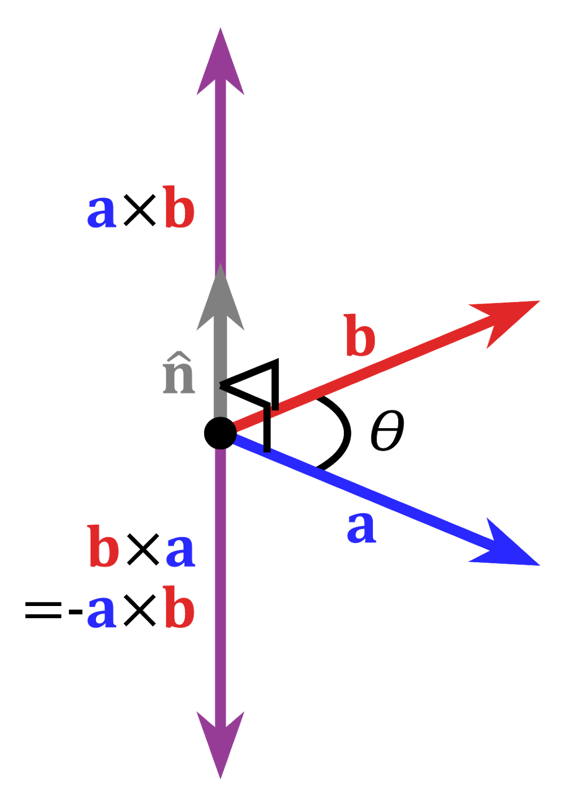

Our cross product term is then written as:

The archetypical cross-product vector is the angular momentum (spin), J.

With an orientation it is known as an axial vector: an orientated line segment perpendicular to the (oriented) plane that describes the rotation of a body around an axis.
A sense is chosen as the left-hand rule in which the thumb directs the axial vector while the middle and forefingers span the support. In picking out a preferred direction we will see, unlike for normal vectors, J remains invariant to an inversion of co-ordinate axis from x to -x. We can think of such vectors, J as generating symmetries and thus conservations laws of our system. They are also observables for the same reason.
Some examples of orientation ¨aware¨ systems are cited below.
A non-chiral (i.e. parity symmetric preserving) theory is called a vector theory. The terms chiral or vector derive from the types of invariant objects that arise from the Representation of the underlying theory's Group of symmetries. In this sense the familiar "vectors" of three-dimensional space are the objects that are invariant -staying the same -when the underlying basis (co-ordinate axis) set is rotated. That is, the vector expresses the equivalence or indistinguishability of the object under rotations.
Quantum Chromo Dynamics (QCD), the quantum field theory that describes the (non-linear) theory of the strong interaction binding together the quarks of a nucleon is an example of a vector theory since both left and right-handed chiralities of all the quarks appear in the theory, and they couple the same way. The electroweak theory as part of QED controlling radioactive decay is a chiral theory despite one of its invariant objects having both right- and left hands. The object being the mass-less neutrino is described by a so-called Weyl spinor that is invariant under the (double cover) of the Lorentz transformations of Einstein’s Special theory of Relativity.
Just as an electromagnetic wave is an oscillation in the electric and magnetic fields that propagates at the speed of light, so is a gravitational wave is an oscillation in the gravitational field. To generate such waves asymmetric collapses or expansions of matter are required as symmetric collapses cancel out far-field gravity wave formation. Resulting gravitational waves propagate through space-time at the speed of light, distorting space-time as it passed through it.
As other force-carrying particles a gravitational wave has integral spin. Being a spin-2 particle with a quadrupole moment, the gravitational wave, passing through any point in space, would both stretch space in one direction and compress the space in the orthogonal direction.
Gravitational waves if they are second quantizable would be carried by gravitons. A graviton is the excitation in the boson-gravitational field, travelling (according to 2017 results form binary-Neutron star coalescence to 15 orders of magnitude in precision to effectively ) the speed of light. It is a spin-2 particle, the only one, which means that it somehow needs only spin half a revolution before it arrives in the same position. As other force-carrying particles it has integral spin. Being a spin-2 particle with a quadrupole moment, the gravitational wave, passing through any point in space, would both stretch space in one direction and compress the space in the orthogonal direction.
In terms of generating a gravitational wave we have the following distinction from electromagnetism. A static mass generates a static gravitational field, just like a static electrical charge generates a static electrical field. An accelerating charge generates electromagnetic radiation, carried by photons.
However, an accelerating mass generates no gravitational waves, gravitational waves are only generated when the acceleration of the mass is changing. That is when the mass has a non zero “snap” (third order derivative of space”, to the fourth and fifth orders of “Crackle” and “pop”).
Some examples of orientation ¨aware¨ systems are cited below.
Spinor Fermions, Vector Gauge Bosons and Chirality
A non-chiral (i.e. parity symmetric preserving) theory is called a vector theory. The terms chiral or vector derive from the types of invariant objects that arise from the Representation of the underlying theory's Group of symmetries. In this sense the familiar "vectors" of three-dimensional space are the objects that are invariant -staying the same -when the underlying basis (co-ordinate axis) set is rotated. That is, the vector expresses the equivalence or indistinguishability of the object under rotations.
Quantum Chromo Dynamics (QCD), the quantum field theory that describes the (non-linear) theory of the strong interaction binding together the quarks of a nucleon is an example of a vector theory since both left and right-handed chiralities of all the quarks appear in the theory, and they couple the same way. The electroweak theory as part of QED controlling radioactive decay is a chiral theory despite one of its invariant objects having both right- and left hands. The object being the mass-less neutrino is described by a so-called Weyl spinor that is invariant under the (double cover) of the Lorentz transformations of Einstein’s Special theory of Relativity.
The Snap Modes of Vibration of a Gravitational Wave
As other force-carrying particles a gravitational wave has integral spin. Being a spin-2 particle with a quadrupole moment, the gravitational wave, passing through any point in space, would both stretch space in one direction and compress the space in the orthogonal direction.
Gravitational waves if they are second quantizable would be carried by gravitons. A graviton is the excitation in the boson-gravitational field, travelling (according to 2017 results form binary-Neutron star coalescence to 15 orders of magnitude in precision to effectively ) the speed of light. It is a spin-2 particle, the only one, which means that it somehow needs only spin half a revolution before it arrives in the same position. As other force-carrying particles it has integral spin. Being a spin-2 particle with a quadrupole moment, the gravitational wave, passing through any point in space, would both stretch space in one direction and compress the space in the orthogonal direction.
In terms of generating a gravitational wave we have the following distinction from electromagnetism. A static mass generates a static gravitational field, just like a static electrical charge generates a static electrical field. An accelerating charge generates electromagnetic radiation, carried by photons.
However, an accelerating mass generates no gravitational waves, gravitational waves are only generated when the acceleration of the mass is changing. That is when the mass has a non zero “snap” (third order derivative of space”, to the fourth and fifth orders of “Crackle” and “pop”).
 is used and in which the constraint that the dynamical connection is a metric compatible connection
  is put in by hand. The field equations read:

 and spin tensors,
  are given in terms of the three forms
  ,
,  with
with  .
. ") are Lorentzian time-space indices of a freely falling frame.
are Lorentzian time-space indices of a freely falling frame. . They are most elegantly presented as two spinor-valued differential 3-form equations,
 ={\sigma}^{AB}")
 where
where  and
and  are known source quantities.
 . These are the co-frame, verbein objects that are Einstein’s freely falling elevator. This dynamical variable,
  is a Hermitian matrix-valued one-form from which the (real Lorentzian) metric is given as
") ,
,  .
.")
 associated to the spin structure over space-time only acquires the interpretation as spinor indices through the dynamical soldering form,
  . A priori there is no relation between the tangent space and the internal space of the vector bundle
  associated to the spinor structure over space time, M. Rather if a (non compact) spacetime manifold,
  defined on it. A spinor structure,
  is a principal fibre bundle with structure group
 ") , the gauge group for spinor dyads. The (real) space-time manifold carries a
, the gauge group for spinor dyads. The (real) space-time manifold carries a  of B consists of a 2-complex dimensional vector space equipped with a symplectic metric,
  .
. and
and  (complex conjugate)
 ") -valued connection one-forms and the torsion two form denoted as
-valued connection one-forms and the torsion two form denoted as  , the first Cartan structure equation reads
 where
where  denotes the exterior covariant derivative with respect to the
  due to


")
 , has been decomposed into spinor fields of dimension 5,9,1 and 3 respectively , corresponding to the anti-self dual part of the Weyl conformal spinor,
  , the spinor representation of the trace-free part of the Ricci tensor,
  and the Ricci scalar
  , – all with respect to the curvature of the
  arising from the presence of non-zero torsion.
 , defined in terms of the co-frame dynamical variable for mere ease of exposition. As we will see in a later post these objects can be treated as the bona fide, fully chiral dynamical “graviton” field object in tis own right.
,") with
with  representing some matter fields.
_{\mathbb{C}}^-\cong SL(2,\mathbb{C})") connection is not associated to the tangent bundle and is thus not a linear connection but a spinor connection. The variation of the Lagrangian with respect to
connection is not associated to the tangent bundle and is thus not a linear connection but a spinor connection. The variation of the Lagrangian with respect to  (with curvature
  ) so the
  can be decomposed according to

 is the contorsion one form, irreducibly written in terms of totally symmetric and`axial’ parts as
}{}^{C'}.")

=0,")

 by
by  .
.") , a complex (semi)chiral fermion matter Lagrangian,
, a complex (semi)chiral fermion matter Lagrangian,  and a term,
  that ensures the standard Einstein-Weyl form of the field equations,
= i\theta^{A}{}_{A'}\wedge\theta^{BA'}\wedge F_{AB},")
=+\eta^{AA'}\wedge\tilde{\lambda}_{A'}\lambda_{A},")
=\frac{3}{16} \lambda_{A}\tilde{\lambda}_{A'}\lambda^A\tilde{\lambda}^{A'},")

") are the left (resp. right)-handed zero forms.
are the left (resp. right)-handed zero forms. (which does not act on tensors, so for example
 supports only the axial part of the torsion of
 }{}^{C'}.")
 and
and  is hermitian) it proves useful to extend
  . Although it is argued that the spin
  field variables can be taken to be either Grassman [or complex]-valued, in fact the use of complex spin
.} \textit { J. Math. Phys, } \textbf{16}, 2395.")
.\textit{Spinors,Tetrads and Forms (unpublished)}.")
, L157.")
, (1995).")